Dynamic Resource Allocation: Best Practices

If you scale on the wrong signals, you waste money and still miss traffic spikes. In many cloud setups, CPU averages around 10% and memory around 23%, yet teams still hit latency spikes, OOMKilled events, and failed requests when demand jumps.

I’d boil this down to a few rules:

• Use the right signals: match scaling to user impact, not just machine load
• Mix scaling types: scheduled for known peaks, reactive for surprises, predictive for repeat patterns
• Set safe policies: scale out early, scale in slowly, and keep hard min/max limits
• Make traffic land well: readiness checks, warm-up time, and zone spread matter as much as autoscaling
• Keep tuning: review lag, thrashing, latency, and cost after tests and product changes

A few numbers stand out:

• Overprovisioning in a 1,000-node setup can cost more than $9.6 million per year
• Predictive scaling can look ahead 15 to 90 minutes
• Baselines should use at least 14 days of data, and 30 days is better
• Scale-down delays often work best in the 5 to 15 minute range
• Deregistration delay should often sit around 30 to 60 seconds

Here’s the core idea: I’d treat dynamic resource allocation as a loop of metrics, decisions, and scaling actions. If any one of those three is off, performance and cost both drift in the wrong direction.

Dynamic Resource Allocation in Cloud Computing | Preetham Vemasani | Conf42 Observability 2024

sbb-itb-18d4e20

Choose Metrics That Reflect Real Application Demand

Autoscaling only works when the signal lines up with the demand your app has to handle. CPU tells you about machine load. It does not tell you how users feel the service. That’s why metric choice is the first scaling call that matters.

A payment API should care about p95 response time. A background job processor should care about queue depth. A cache layer should care about memory utilization. Pick the wrong signal, and your scaling system will respond to the wrong problem. Then, when the metric that does matter starts to spike, users may already be feeling it.

Use a Mix of Infrastructure and Service Metrics

No single metric tells the whole story. CPU helps, but it can miss I/O-bound bottlenecks, lock contention, and services that are running into downstream rate limits. Memory is also tricky for autoscaling because it can stay high after load drops, which can leave systems scaling up and never scaling back down.

A safer approach is to combine four signal types: Utilization, Saturation, Latency, and Errors. Use one main signal for each workload, then pair it with one support signal.

There’s one practical detail here that people often miss: scale on 95th-percentile node CPU, not the fleet average. Averages can smooth over hot spots and hide overloaded nodes. If a service starts to degrade at 85% CPU, set the scaling target around 60%. That 20 to 30 percentage point buffer gives new capacity time to come online before users notice a slowdown.

Validate Baselines Before Enabling Automation

Before turning on any automated scaling policy, you need a clear picture of what “normal” looks like for that workload. In practice, that means collecting data for at least 14 days, and ideally 30 days, so you can see a full business cycle.

During that period, track response times in milliseconds at p95 and p99, along with request volume in requests per second (RPS). Then calculate your peak multiplier by dividing peak RPS by baseline RPS. That gives your scaling policy room for peak demand instead of tuning it only for steady-state traffic.

Use that baseline data to check one simple thing: does the metric move when customers feel pain? This matters most in checkout, payment, and API paths. If the metric doesn’t move with customer pain, don’t use it to drive scaling.

These baselines become the thresholds used in the next policy layer.

Design Scaling Policies That Prevent Waste and Instability

Once you have solid baselines and the right metrics in place, policy design is the next layer. This is where teams either build a steady system or end up with one that flaps, overreacts, and leaves users exposed when traffic shifts all at once.

Set Thresholds, Cooldowns, and Capacity Limits

Use your baseline metrics to decide when scaling starts, how long it waits, and how much spare room it keeps.

The basic rule is simple: scale out fast and scale in slowly. A short period of extra capacity usually costs less than an outage. Set your scale-out threshold 20 to 30 percentage points below the point where the service starts to struggle. For cooldowns, the scale-up cooldown should roughly match the time new capacity needs to become healthy. The scale-down cooldown should be 5 to 15 minutes so you don't remove capacity right before traffic comes back.

If traffic is noisy or spiky, a stabilization window often works better than a plain cooldown because it uses the lowest safe recommendation across a window.

You also need hard limits. Set a floor so a single-node failure doesn't knock the service over. Two replicas is the practical minimum for most services, and three is the better choice for services with strict SLAs. Then set a maximum capacity ceiling to guard against budget overruns and runaway retries. Those guardrails keep scaling safe. After that, the next job is deciding how traffic lands on that capacity.

Layer Scheduled Rules on Top of Real-Time Policies

Schedule capacity for demand you can predict, then let real-time rules handle the spikes you can't.

Use schedules for known peaks and keep reactive rules for everything else. This works well for repeating patterns like business hours and planned events.

When building a schedule, provision for expected average demand plus a 20% safety buffer. Also set schedule lead time to at least 5 minutes so capacity is fully initialized before traffic arrives. Then use target tracking so reactive scaling can fill the gap between scheduled capacity and live demand.

Balance Traffic and Compare Scaling Approaches

Load balancing decides whether new capacity can actually take traffic. Autoscaling may add instances, but the load balancer is what turns that extra capacity into something your users can use.

Distribute Load Across Healthy Capacity

After you add capacity, the next job is simple: send requests to the right place. That means using readiness checks, not just basic pings. Traffic should go only to instances that pass readiness checks, not only liveness checks. An instance can be alive but still not ready to serve requests, and sending traffic there can lead to silent failures.

Use Layer 7 application balancers for HTTP services that need routing logic. Use Layer 4 transport balancers for non-HTTP traffic that needs lower overhead.

Two traffic distribution problems show up all the time.

First, sticky sessions can create hot spots when too many requests stay stuck to the same nodes. If you need session persistence, move session state to a shared store like Redis so any node can handle the request.

Second, spread replicas across Availability Zones with anti-affinity rules. That way, one zone issue doesn't wipe out too much capacity at once. And if a single load balancer hits its own limit, split traffic across multiple balancers with weighted DNS.

When new capacity comes online, don't send production traffic to it too early. Use startup grace periods and warm-up settings so the app, caches, and JIT compilation have time to get ready. On the way down, use a deregistration delay of 30–60 seconds so in-flight requests can finish before an instance is removed.

Once routing is steady, the next step is picking the scaling method that fits the bottleneck.

Horizontal vs. Vertical vs. Node-Level Scaling

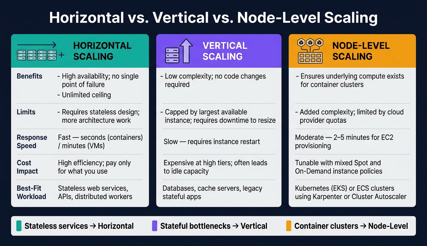
Pick the scaling method based on the bottleneck, not just the way the app is deployed.

A simple way to think about it:

• Use horizontal scaling for stateless services.
• Use vertical scaling for stateful bottlenecks.
• Use node-level scaling for container clusters.

Next, watch how these options hold up under live traffic.

Monitor, Test, and Tune Continuously

Once policies are live, you need to check whether they still fit current demand. After scaling goes live, the work moves from setup to verification.

Use Alerts, Dashboards, and Historical Reviews

Track whether the scaling signal still lines up with actual user pain. Also watch for drift between load, latency, and scaling actions. Two failure patterns matter most here: thrashing - repeated up-and-down scaling - and scaling lag - the delay between a breach and usable capacity.

Tag resources by team, project, and environment so cost reviews are easy to run and easy to act on. For stable workloads, review behavior every quarter. For fast-growing systems, check monthly or on a continuous basis.

Once you can see scaling behavior clearly, cost data tells you whether the policy is efficient or just stable. Use latency histograms and node saturation rates to catch drift in thresholds. Common visibility stacks include Prometheus and Grafana for metrics, plus Datadog or New Relic for full-stack observability and distributed tracing. Different tools, same job: show saturation, failed scale events, and cost drift in one place so problems don’t slip through.

Retune Policies After Load Tests and Architecture Changes

When the workload changes, don’t assume the old thresholds still work. Retest first. Run ramp, spike, and soak tests to see how the system reacts to different traffic patterns. Those tests also show whether your horizontal, vertical, or node-level scaling plan can handle real demand.

A simple way to do this: start with fixed resources, then keep increasing demand until performance drops. That breakpoint shows your actual headroom. After each test, review p50, p95, and p99 latency histograms along with CPU throttling metrics like container_cpu_cfs_throttled_seconds_total and cost per 10,000 requests.

Go back to scaling rules after any major feature launch, traffic shift, or architecture change. Once traffic settles after a release, recheck thresholds. Stable workloads should still be reviewed quarterly, while fast-growing products should move to monthly or continuous automated reviews. Regular tuning cuts waste and helps keep performance steady.

FAQs

How do I pick the best scaling metric?

Choose your scaling metric based on how your app behaves. There isn't one best metric for every case.

For latency-sensitive services, request latency is usually the clearest signal. If your app works through a backlog, queue size is often the metric you can trust most. For standard web apps, CPU utilization is a common pick, but leave 20% to 30% headroom so the system isn't running too close to the edge.

Try not to use memory as your main metric. It can make scale-down harder than it should be. It's also smart to use at least two signals instead of relying on just one, then test your thresholds against your performance goals.

When should I use scheduled vs. reactive scaling?

Use scheduled scaling when traffic tends to follow a pattern, like daily busy hours or planned marketing campaigns. Provisioning can take anywhere from seconds to minutes, so setting capacity ahead of time helps make sure resources are in place before demand shows up.

Use reactive scaling when workloads are less predictable and can spike out of nowhere. In practice, many teams use both: scheduled scaling for expected demand, and reactive scaling as a backup for sudden surges.

How can I stop autoscaling from thrashing?

Use stability guardrails so autoscaling doesn’t swing with every short spike or dip. Set stabilization windows so metrics need to stay high or low for a bit before a scaling action happens. This matters even more for scale-down, where cutting capacity too fast can hurt performance. Add cooldown periods too, so new instances have time to warm up and carry traffic before the system makes another change.

It also helps to base scaling triggers on leading signals like queue depth or latency targets instead of lagging metrics like CPU or memory. CPU often tells you a problem is already happening. Queue depth and latency usually give you an earlier heads-up. And one more thing: avoid running conflicting autoscaling policies on the same resource, or the system can end up fighting itself.